The recent bushfire activity in Australia reminded me of an interesting problem in statistical physics, and a model that somewhat resembles the spread of a forest fire.
Percolation
Percolation describes the process of fluid movement through a porous medium. Besides their direct application in fluid dynamics and material science, percolation models have been used to study various phenomena across a diverse set of applications, ranging from epidemiology and financial markets to forest fires.
Percolation models are relatively easy to define and construct, but show interesting behaviour linked to phase changes, like fractal dimensions, scaling behaviour and power laws.
A simple forest fire model
Let’s assume we have a square lattice of length n. Every square of the lattice can either be occupied by a tree with probability p, or be empty with probability (1-p). Assume the trees in the top row of the lattice are set on fire, and that the fire will spread to directly neighbouring trees over time. What’s the probability that the fire will reach the lower end of the lattice given enough time? (The correct academic expression for this model is “site percolation on a square lattice”.)
Intuitively, the probability depends on the amount of trees and how the trees are clustered across the lattice. If there were no trees, the probability would be 0, and if every site were occupied by a tree, the probability would be 1. How does this probability behave for p in between these two extremes?
To solve this problem, we’ll use a simulation approach: Simulate the system many times over for p values between 0 and 1, and compute the probability that the fire reaches the bottom row for each p through sample statistics. For the simulation we’ll set the lattice size n to 400 (the bigger the better).
An algorithm to solve this model closely resembles the spreading dynamics of a forest fire:
- Initialize the lattice and on each lattice square plant a tree with probability p.
- Set the top row of trees on fire
- In each time step, set all trees next to the burning trees on fire, and set the already burning trees’ status to burnt.
- Continue until no more trees are burning or the fire reaches the bottom end.
The lattice is traversed in an approach that is very similar to breadth-first-search in graph theory.

Before looking at the solution, take a guess how the probability of the fire spreading to the bottom row depends on the value of p. Are you expecting a linear increase of the probability with increasing p?
Result


The probability of the fire reaching the bottom end of the lattice is zero below 0.5, jumps to one above 0.6, and the sample variances are very small. Highly suspicious! In fact, if we were able to simulate the system for an infinitely large lattice, we could see that at approximately p=0.59 the probability of the fire reaching the bottom row jumps from 0 to 1. This discontinuity is smeared out in our results due to the finite lattice size we use in our simulation. It turns out that 0.59 is a so called critical point of the system, 
- The probability of a spanning cluster (a connected cluster connecting the top and bottom, i.e. the probability that the fire reaches the bottom) jumps from 0 to 1.
- The shortest path from top to bottom reaches its maximal length.
- The spanning cluster has a fractal dimension.
- The probability of a site of the lattice being part of the spanning cluster can be described by a power law when p is close to
- The cluster size distribution (number of independent clusters in the lattice with a given size) follows an inverse power law.
Effectively, the system is undergoing a phase transition at
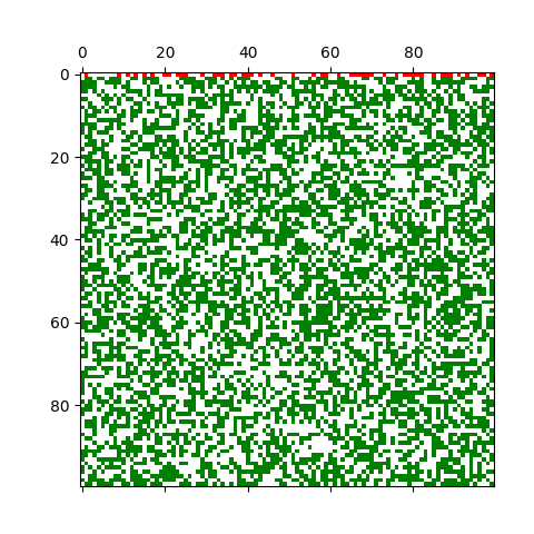
 for N=200. There remain large patches of unburnt trees, and the fire spreads very slowly.
 , and then decays towards the lattice length of 400.
I’m always amazed how such simple systems can lead to such complex dynamics.
Implementation side note
The code is available on GitLab here. My previous implementation was in C++, but here I wanted to write a pure and well-understandable python implementation of the algorithm. The drawback of this approach is the loss of speed – the code continually loops over all cells using standard for-loops which is known to be very inefficient. To speed up the code, I used Numbas JIT compilation, which increased the speed by more than a factor of 100. It would be interesting to see how a cythonized, a vectorized (using numpy), and the numba version compare versus a raw C++ code… in a future blog post.
